Effect of Elephant Paths on Orienteering Performance

Introduction

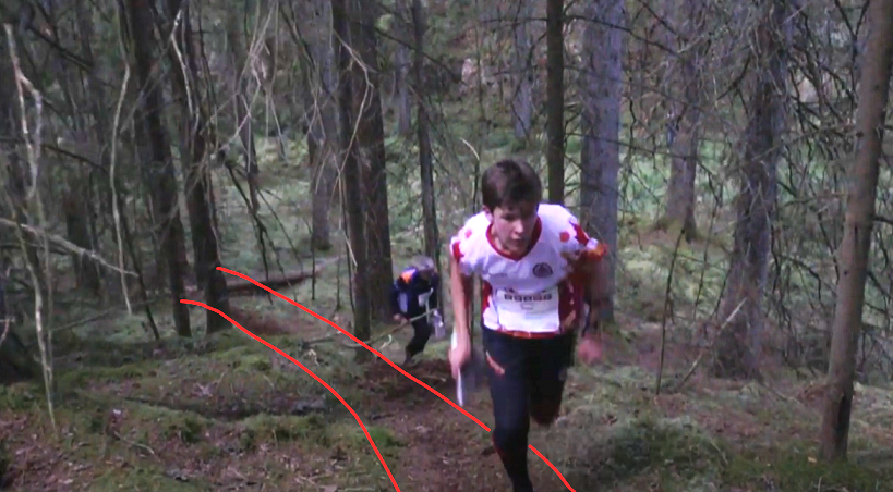
Orienteering is a sport which combines running with precision navigation using map and compass. Athletes must execute the best route between a series of points, called “controls”, dispersed through a forest or city. To discourage following, orienteers typically start at intervals of 1-3 minutes. However, when several orienteers run the same “leg” (two consecutive controls, the time between which is known as a “split”), paths may form through the forest along the fastest routes. In Orienteering parlance, these are commonly referred to as “elephant paths”. An example of an orienteer running along a such an elephant path is shown below (source).

It has long been suspected among orienteers that these elephant paths confer an advantage to later runners, as they aid in both navigation and running. This article presents an attempt to quantify this advantage, using data from the largest multi-day orienteering event in the world, Oringen.

Data Source

I chose Oringen as the data source for this project for two main reasons:

1. Large datasets (Oringen attracts 12,000 to 20,000 orienteers annually)
2. Pseudo-random start times over 4 days of competition

Most elite competitions in orienteering have seeded starts, which means that higher-ranking athletes start towards the back of the field. This makes it difficult to separate natural performance from advantages due to elephant paths. At Oringen, competitors are assigned to one of four start blocks on each day of competition, starting in one of each over the four days of competition. The fifth day is a chase-start and is excluded from this analysis.

Elite classes also have some type of seeding at Oringen, so have been excluded. The rest of the classes are included as “random” if they meet the following criteria:

1. 30 or more competitors
2. There is less than a 60% chance that a randomly chosen competitor starts in the same half of the start window on two randomly selected race days

I used data from 13 Oringens between 2010 and 2024. When broken down into individual legs for individual runners, this amounts to 4.25 million rows of data.

Methodology

The basic question we want to answer is this: When an orienteer starts on a leg, is there a correlation between the number of orienteers who have already run that leg, and that orienteer’s split for that leg? We’ll introduce a new term here to simplify this text going forward: if I’m the 67th person to run a particular leg, my “split order” is 67.

Since we can only guarantee a pseudo-random distribution of skill level within a class, I normalized an athlete’s split for each leg to the mean of their class’s time on that leg. Keep in mind this means a lower number is better. It is still somewhat problematic to compare these normalized performances between classes, since classes arriving at a control at different points in their race will have a different mean “split order”. If our hypothesis is correct, that split order is correlated to performance, then we will be normalizing to different “levels” of performance in different classes. While we might be normalizing the performance of Class A about a split order of 55, we might be normalizing the performance of Class B about a split order of 107. This is mitigated to some extent by Oringen’s large and numerous categories, and long start windows.

As for calculating the split order itself, further problems arise. If we simply take the order as described, using the timestamp of when an orienteer begins that leg, we are inherently introducing a bias towards natural performance that we sought to eliminate by using only pseudo-random start times. Given the same start time, a worse orienteer will arrive at a control later, and hence have a higher split order. This might introduce a false trend towards worse performance at higher split orders.

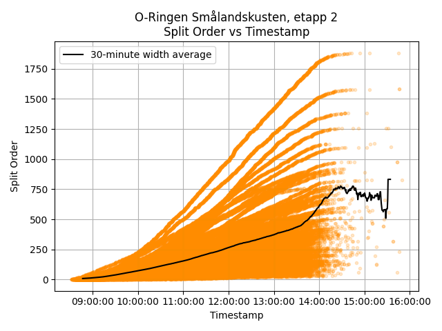
Conversely, if we take the split order as it exists for each leg when the athlete starts, we will distort any resulting correlations. As seen in the example below, the split order does not increase linearly over the course of the race day, and instead follows an “S” curve. The different magnitudes of split orders are due to the fact that some legs are shared among multiple classes.

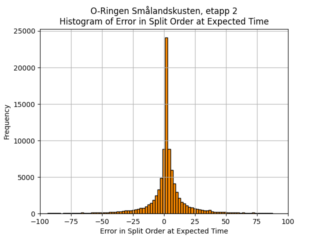
A compromise is to calculate the time that an athlete “should” have reached a given leg based on the mean time to reach that leg in their class. We then calculate the split order they would have had under this scenario, and use this as the x-axis value for their split performance. A histogram of the error in this “pseudo split-order” shows a fairly normal distribution, but it is worth noting that this step increases the magnitude of the relationship between split order and split performance. The expected split order will be lower than the actual split order for poorer performing athletes, and vice-versa for higher performning athletes. This has the effect of increasing the negativity of any trend. So while using the “true” split order biases towards natural ability, this may bias too far in the other direction, leading to an over-estimation of the effect of elephant trails.

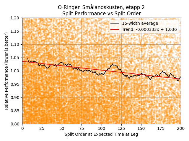
We can now move on to plotting our split performance against the pseudo split order. An example is shown below, including split orders up to 1500.

As the number of splits thins out, the noise becomes very large. If there is an advantage, it must level out at some point, but it’s hard to discern. Moreover, for most competitions we are not interested in the change of performance between the 1000th and 1500th person to run a particular leg. For elite competitions, the athlete pool is often restricted below 200 competitors anyway. I therefore cut the maximum split order considered down to 200, and plotted a linear trend line through this data.

The trends for all 52 races are shown below:

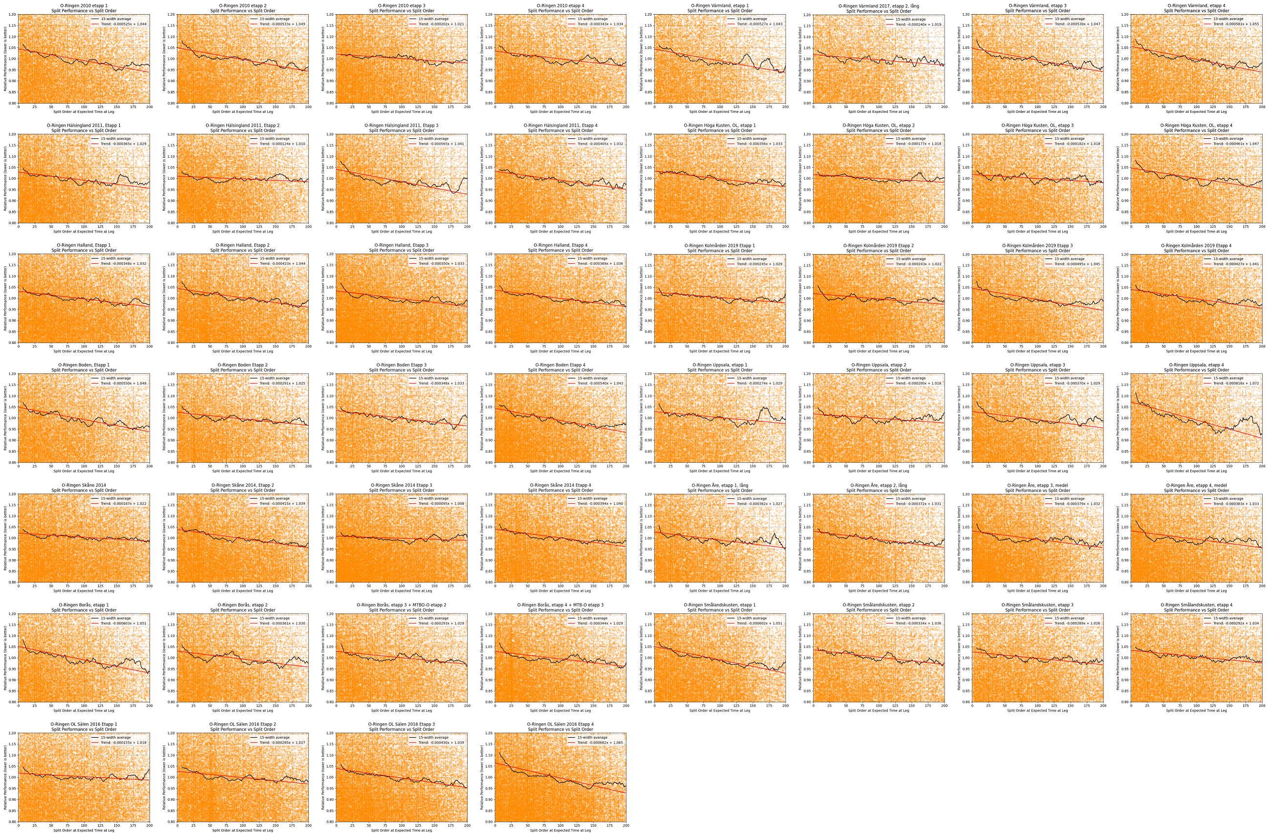
Results

For each race, I normalized the performance trend to a split order of 0, meaning that performance gains are represented as an advantage over an orienteer running through untouched terrain. Then taking the average of all trend lines (52 races in all), I obtained an average relationship of -0.000364 with standard deviation 0.000137. This indicates that all else equal, the 100th runner on a leg would, on average, be 3.6% faster than they would have been had they started first. The 200th runner has a 7.3% advantage.

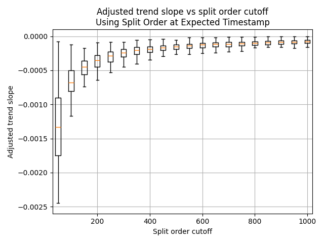
Cutting off the split order at 200 was of course an arbitrary decision, so it’s worth examing how the results change if we modify this cutoff. The following plot shows boxplots of the adjusted (i.e., normalized to a split order of 0) trend line slopes for split order cutoffs from 50 to 1000. As expected, the trend is more dramatic for lower split orders, and starts to level off as we include higher split orders. This indicates that the incremental advantage confered by prior runners on a leg is greatest for the first few competitors, then diminishes. Slopes for split order cutoffs lower than 200 can be gleaned from this graph, but the uncertainty becomes larger.

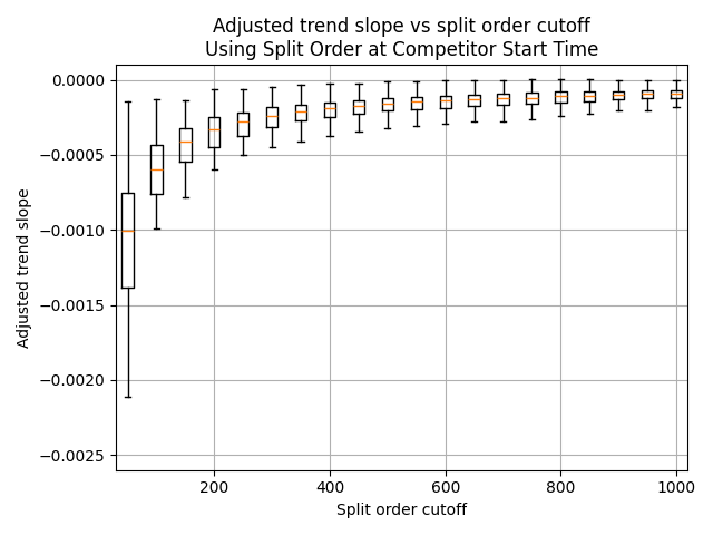
Given the possible over-estimation of the slope using the split order at expected timestamp, as mentioned above, it may also be worth looking at the results using split order at start time. In this case, the slope for a split order cutoff of 200 is slightly diminished, at -0.000346, with standard deviation 0.000142. For completeness, the same boxplot is generated below:

Confounding factors/further research

1. A major downside of using Oringen as a data source is that arenas are often re-used between races. Hence, some legs that are reset to a split order of 0 for day two may in fact be identical to legs from the previous day’s race. With no master maps from the competions included in this analysis, I made no attempt to correct for this. Re-doing the analysis with only the 13 first-day races, with a split order cutoff of 200, I find a mean relationship of -0.000393 (std dev 0.000128). This slightly higher performance boost for later runners indicates that stadium re-use may be having some effect.

2. Heat affects runners’ performance. Since the competitor start window is several hours long, orienteers are exposed to different weather conditions on course. It would be interesting to see if increasing temperatures can be found to correlate with poorer performance for later runners, but given the noise in the data this effect may be too small to find.

3. Orienteers know that elephant paths can make a bigger difference in some terrain over others, particularly when there’s heavy understory. This could help explain the large standard deviation seen in the trend slope lines, and would also be an interesting avenue for further exploration, although collecting a reliable dataset may prove challenging.

4. All this analysis excludes data from elite runners. If elite runners benefit to a different extent from elephant trails than the general orienteering population, the conclusions drawn here may not be applicable to elite fields.

5. Given the changing slopes of the trend lines in the results section, it would be interesting to fit a non-linear trend to the data, such as an exponential decay with a type of offset. This hasn’t been attempted here due to the difficulty of combining the trends of multiple data series.

Updates

2025-01-03: Added box plots to show the changes in trend line slopes depending on split order cutoff, and added a bit more discussion of possible flaws in the methodology